
Slippage Analysis Trading: A Quant's Practical Playbook


Slippage analysis trading is the systematic process of measuring the gap between your expected execution price and the price you actually received, then using that gap to benchmark, model, and reduce execution costs. The three actions to run right now: (1) record the National Best Bid and Offer (NBBO) at the exact moment you submit each order, (2) log every fill with its timestamp and partial-fill breakdown, and (3) pull a 50–100 trade sample and segment it by product, time of day, and order type to surface systematic patterns, as Pomegra’s execution library recommends.
For benchmark selection: use NBBO if you trade fast intraday momentum where microseconds matter, use the midpoint for a spread-agnostic comparison that strips out half the bid-ask cost, and use VWAP when your fills are algorithmic and sized relative to market volume. Discipline AI’s execution-quality scoring can instrument all three automatically, so you are not doing this in a spreadsheet indefinitely.
Record NBBO at order submission (not at fill time)
Log every fill: timestamp, price, size, venue, order type
Run your first 50–100 trade sample segmented by product, time, and order type
Key Takeaways
Slippage analysis trading requires clean fill-level data benchmarked to NBBO or VWAP, a time-aware modeling workflow, and execution tactics applied at the pre-trade, intra-trade, and post-trade stages.
Point | Details |
Benchmark selection matters | Use NBBO for intraday speed, midpoint for spread-agnostic comparison, VWAP for algorithmic execution. |
Start with 50–100 fills | Segment by product, time of day, and order type to surface systematic slippage patterns before modeling. |
Order size drives impact | Keep each slice below 10–15% of visible book depth to avoid nonlinear price impact. |
Time-series CV is non-negotiable | Use blocked or expanding-window cross-validation; standard k-fold leaks future data into training. |
Disciplineaiapp automates the loop | Execution scoring, automated autopsies, and slippage dashboards replace a custom data pipeline. |
Table of Contents
How to measure slippage: benchmarks, formulas, and a worked example
Which data sources actually give you reliable slippage estimates
How to model slippage statistically and with machine learning
Concrete tactics to reduce realized slippage before, during, and after a trade
How to inject slippage into backtests without introducing bias
How Disciplineaiapp instruments slippage and closes the execution loop
Disciplineaiapp gives you execution scoring without building a pipeline from scratch
What causes slippage and how to classify it
Slippage is the realized execution difference between the price you expected when you placed the order and the price the market gave you. Three distinct types appear in practice, each pointing to a different fix.
Price slippage happens when the market moves between your order submission and its fill. A fast-moving BTC/USD pair during a news print is the textbook case: you submit at $65,000, the book shifts, and you fill at $65,180.
Time slippage (latency) is the cost of delay. Your order sits in a queue, the price drifts, and by the time the exchange processes it, the level you wanted is gone. Co-location and VPS setups exist specifically to compress this window.
Implementation shortfall is the broadest measure. It captures the full cost of going from a decision price (the mid when you decided to trade) to your final average fill, including both price movement and market impact from your own order consuming book depth.
Primary causes, ranked by how often they dominate:
Order size vs. available depth: a large order hitting a book with thin depth at the best ask will walk up the price ladder. The impact scales nonlinearly with order size relative to visible depth.
Volatility and news events: realized volatility spikes widen spreads and thin books simultaneously. Clustered large fills at the open or close are a reliable flag that you are trading in a high-slippage window.
Bid-ask spread: as Nadcab’s breakdown of execution costs clarifies, spread is the visible static cost, price impact is the deterministic cost from consuming depth, and slippage wraps both plus unpredictable market movement. Conflating them leads to bad model specs.
Latency and routing: every millisecond of extra round-trip time is an opportunity for the book to move. Smart-order routing that adds hops can add slippage even on liquid instruments.
Market microstructure events: opening auctions, index rebalances, and exchange-level outages create temporary book dislocations that look like outlier slippage but are actually regime events. Flag these separately rather than letting them distort your baseline.
How to measure slippage: benchmarks, formulas, and a worked example
Benchmark selection is the first decision. NBBO suits intraday equity and crypto traders who need a real-time reference. Midpoint strips out the spread and is useful when comparing execution quality across venues with different tick sizes. VWAP is the right benchmark for algorithmic execution where you are trying to minimize market impact over a time window.
Core formulas:
Per-trade slippage (in dollars):
Slippage ($) = (Fill Price − Reference Price) × Signed Direction × Shares/Contracts
Where Signed Direction = +1 for buys, −1 for sells (so adverse slippage is always positive).
Per-trade slippage (in basis points):
Slippage (bps) = [(Fill Price − Reference Price) / Reference Price] × 10,000 × Signed Direction
Implementation shortfall:
IS = (Average Fill Price − Decision Midpoint) / Decision Midpoint × 10,000 × Signed Direction
Worked order-book example:
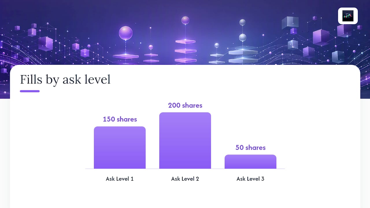
You want to buy 400 shares. The L2 book at submission shows:
Ask Level | Price | Size |
Level 1 | $100.10 | 150 shares |
Level 2 | $100.15 | 200 shares |
Level 3 | $100.22 | 400 shares |
Your 400-share market order fills as: 150 @ $100.10, 200 @ $100.15, 50 @ $100.22.
Volume-weighted average fill price:
VWAP fill = [(150 × $100.10) + (200 × $100.15) + (50 × $100.22)] / 400 = [$15,015 + $20,030 + $5,011] / 400 = $40,056 / 400 = $100.14
If the NBBO midpoint at submission was $100.05:
Slippage = ($100.14 − $100.05) / $100.05 × 10,000 = 9.0 bps
Coin Metrics publishes hourly liquidity slippage metrics using exactly this approach for fixed USD order sizes (1K, 5K, 10K, 100K), reporting null when book depth is insufficient to fill the order.
Implementation notes for code: capture the order submission timestamp and the NBBO snapshot at that exact microsecond, not at fill time. For partial fills, compute a weighted average across all child fills before comparing to the reference. Include exchange fees in a separate field so you can report gross and net slippage independently. OANDA’s execution risk guide treats slippage as an inevitable variable cost, which is the right mental model: budget it, measure it, and reduce it systematically.
Which data sources actually give you reliable slippage estimates
Not all data is equal for fill simulation. Here is how the tiers stack up, from most to least useful:
Full L2 order-book events (best): every add, cancel, and modify at each price level. Lets you reconstruct the exact book state at submission time and simulate fills deterministically. The tradeoff is data volume and storage cost.
L2 snapshots at fixed intervals: practical for most teams. Capture depth at 100ms or 500ms intervals. You lose intra-snapshot microstructure but retain enough to estimate price impact for orders up to a few percent of visible depth. Null values when depth is insufficient should be flagged, not imputed.
Trade prints (time-and-sales): show what actually traded, not what was available. Useful for reconstructing realized slippage empirically but cannot tell you what the book looked like before your order arrived.
Reconstructed NBBO: synthesized from exchange feeds. Good for benchmarking but introduces aggregation latency that can misalign timestamps by tens of milliseconds on fast instruments.
OHLCV (weakest): bar-level data cannot support fill-level analysis. Use it only for long-window liquidity proxies like average daily volume ratios. For order-flow analysis, you need at minimum trade prints.
Pseudo-algorithm for simulating a market order against an L2 snapshot:
Sort ask levels ascending (bid levels descending for sells).
Walk the book: subtract available size at each level from remaining order quantity.
Record the price and filled quantity at each level.
Compute VWAP across all filled levels.
If remaining quantity exceeds total visible depth, flag as “insufficient depth” and report partial fill only.
Practical data quality issues to handle: timestamp alignment across venues can drift by 1–5ms on crypto exchanges, which matters for NBBO reconstruction. Synthetic aggregated NBBO from data vendors may lag real exchange feeds. Always validate your pipeline by comparing simulated fills against a sample of actual fills before trusting model outputs.
The QuantJourney slippage-analysis.py script on GitHub implements basic slippage calculations and VWAP-style fill simulation and is a solid starting point for building your own pipeline.
How to model slippage statistically and with machine learning
A modeling workflow that actually generalizes follows this sequence: feature engineering, candidate model selection, time-series cross-validation, and evaluation against held-out regimes.
High-impact features to engineer:
Trade size as a fraction of visible book depth (the single most predictive feature in most liquid markets)
Bid-ask spread at submission (absolute and relative to recent average)
Order book slope: depth-weighted price change per unit of size consumed
Recent trade imbalance: buy volume minus sell volume over the last N seconds
Realized volatility over the last 5 and 30 minutes
Top-of-book change rate (how fast the best bid/ask is moving)
Time-of-day and day-of-week flags
Venue and instrument flags
Model families to try, in order of complexity:
Start with a regularized linear model (Ridge or Lasso). It is interpretable, fast to retrain, and often competitive with more complex approaches on out-of-sample slippage buckets. Add a gradient-boosted tree (XGBoost or LightGBM) to capture nonlinear interactions between spread and volatility. Simple neural nets rarely outperform gradient boosting on tabular execution data unless you have millions of fills.
Validation must be time-aware. Standard k-fold cross-validation leaks future data into training folds. Use blocked or expanding-window CV: train on the first N months, validate on month N+1, then roll forward. Test separately on stressed regimes (high-volatility periods, liquidity events) to confirm the model does not collapse when conditions change.
Evaluation metrics to track:
MAE and RMSE on held-out fills
Directional calibration: does the model correctly predict which fills will be worse than the median?
Implementation shortfall distributions: compare predicted vs. realized IS percentiles
Percentile summaries (50th, 90th, 95th) to catch tail behavior
Pro Tip: A calibrated quantile regression on top of a simple regularized linear model often beats a complex black-box for out-of-sample slippage buckets. The quantile layer gives you prediction intervals, which are more useful for execution decisions than a point estimate.
Nonstationarity is the main modeling risk. Market microstructure changes after major venue upgrades, regulatory shifts, or sustained volatility regime changes. Retrain on a rolling window and monitor feature drift.
Concrete tactics to reduce realized slippage before, during, and after a trade
Mitigation works at three stages. Most traders focus only on execution; the biggest gains usually come from pre-trade sizing decisions.
Pre-trade:
Keep each order slice below 10–15% of visible depth at the best level. Above that threshold, price impact scales sharply.
Check the spread relative to its 30-day average before sending. If it is more than 1.5x the average, either wait or use a limit order.
Avoid trading in the first and last 5 minutes of a session unless your strategy specifically requires it. Spreads are widest and book depth is thinnest at those windows.
During execution:
Use limit orders for entries where fill certainty is not critical. Stop-limit orders over plain stops prevent runaway fills during fast markets.
For larger orders, slice into child orders and use TWAP when you want even time distribution, VWAP when you want to track market volume, or POV (Percentage of Volume) when you want to cap your participation rate.
Randomize child order timing and size slightly to avoid telegraphing your intent to market makers.
Route to deeper venues first. Monitor hidden liquidity using iceberg detection tools. Liquidity void conditions require either smaller slices or a full stand-aside.
Post-trade:
Log every fill at the child-order level. Aggregate fills that belong to the same parent order before computing slippage against the decision price.
Set automated alerts for any fill where realized slippage exceeds your 90th-percentile threshold. These outliers usually point to a specific venue, time window, or order type.
When your slippage model shows drift (predicted vs. realized diverging by more than one MAE unit for 10 consecutive fills), trigger a parameter review.
Liquidity sweep entries are a practical example of pre-positioning to reduce adverse slippage: entering at a sweep level rather than chasing the move means your reference price is closer to your fill.
How to inject slippage into backtests without introducing bias
A backtest that ignores slippage overstates returns. One that uses a flat per-trade cost underestimates tail risk. The right approach combines a deterministic price-impact term with a stochastic residual.
The recipe:
Compute the book-derived VWAP fill for each simulated order using the L2 snapshot at the decision bar’s close (or the nearest available snapshot).
Add a stochastic residual sampled from your historical residual slippage distribution, segmented by hour and liquidity bucket. This captures the unpredictable market-movement component that the book-impact model misses.
Pomegra’s backtest guidance recommends this hybrid approach to avoid both overly deterministic and overly optimistic simulations.
Biases to eliminate:
Lookahead bias: never use the fill price from the bar that triggered the signal as your entry price. Use the next bar’s open or a simulated book fill.
Survivorship bias: if your instrument universe excludes delisted or halted assets, your slippage estimates will be too low because those assets tend to have the worst execution.
Timestamp misalignment: signal generation time and order submission time are not the same. Model the latency gap explicitly.
Future market-state features: do not use features computed from data after the decision timestamp in your slippage model.
Validation sequence: run walk-forward tests with at least 6-month out-of-sample windows. Test separately on stressed periods. Before full live deployment, run a paper-trading or A/B trial where half your orders use the new execution parameters and half use the baseline. Report realized slippage percentiles, implementation shortfall mean and median, and the cumulative P&L delta attributable to execution changes. Use backtesting software that supports custom slippage injection rather than fixed-cost approximations.
How Disciplineaiapp instruments slippage and closes the execution loop
Disciplineaiapp’s platform handles the instrumentation layer that most traders build manually and inconsistently. The relevant features for execution quality work:
Execution-quality scoring: each fill receives a score benchmarked against NBBO, midpoint, and VWAP so you can compare across instruments and time windows without building your own benchmark pipeline.
Automated trade autopsies: after each trade closes, the platform segments the fill-level data by time of day, order type, and market structure condition to surface the specific cause of adverse slippage.
Market structure and liquidity event detection: the platform flags when book conditions shift (spread widening, depth thinning, liquidation cascades) so you can apply stand-aside protection before sending orders into a deteriorating book.
Trade journaling and performance analytics: fill-level logs feed directly into execution performance dashboards that track slippage trends over time.
A practical workflow: monitor fills in real time → run an automated autopsy after each session segmented by product and order type → update your slippage model with the new fill data → push revised execution parameters (slice size, timing, venue preference) to your algo or manual rules → monitor the effect over the next 50 fills. The loop closes without requiring a separate data pipeline or custom dashboard.
Slippage reduction in practice: examples across markets
Shifting order submission to 9:45 AM ET and switching from market to limit orders with a 2-bps tolerance reduced average slippage from roughly 4 bps to under 2 bps on that segment, with minimal impact on fill rate.
Crypto perpetuals: on BTC/USD perpetuals, order size relative to visible depth is the dominant driver.

Forex spot (retail): in forex trading, slippage is heavily influenced by the dealing desk or ECN model. Switching from a market maker to an ECN venue with direct market access reduced average slippage on EUR/USD during news events, where the market-maker model widens spreads aggressively. Timing trades away from major data releases (NFP, FOMC) and using stop-limit rather than plain stop orders are the two highest-leverage changes for most retail forex traders.
Futures (ES, NQ): for CME equity index futures, the primary slippage driver during normal hours is order size relative to the visible bid or ask. A 10-lot order on ES during regular trading hours typically fills at or near the best level. The same 10-lot order sent 30 seconds before a major economic release can walk 2–3 ticks. Pre-trade volatility screening that blocks order submission within a configurable window before scheduled releases is a standard mitigation in professional execution systems.
What I actually prioritize when working on slippage
Most teams spend too much time on the model and not enough on the data pipeline. A clean, timestamp-aligned fill log with NBBO snapshots at submission time is worth more than a sophisticated gradient-boosted model trained on dirty data. Get the instrumentation right first.
My prioritization order: instrument the data pipeline → establish a baseline on 50–100 fills → run small experiments (one variable at a time: order type, timing, slice size) → productionize the changes that show consistent improvement → then build a model to predict which fills will be worst so you can apply tighter controls selectively.
Where to spend your time and engineering effort:
50–100 trade sample with NBBO at submission: one weekend of work, immediate diagnostic value
Fill-level logging pipeline: 1–2 weeks of engineering, permanent infrastructure
Simple regularized model plus live slippage gauge: 2–4 weeks, meaningful signal
Automated parameter tuning: only after the model has proven stable over at least 200 out-of-sample fills
On the build-vs-buy question: if your fill volume is under 500 trades per month, a spreadsheet-based approach with manual NBBO logging is viable. Above that, the engineering cost of a custom pipeline starts to compete with the cost of a platform that already has the instrumentation built. OANDA’s framing of slippage as a budgeted variable cost is the right mindset: the goal is not to eliminate it but to reduce it below the threshold where it materially affects your strategy’s edge.
Disciplineaiapp gives you execution scoring without building a pipeline from scratch
Execution quality measurement is the part of trading infrastructure that most active traders defer indefinitely because building it from scratch is genuinely time-consuming. Disciplineaiapp removes that barrier: the platform delivers fill-level execution scoring, automated trade autopsies, and slippage trend dashboards out of the box, so you start with a working baseline instead of a blank spreadsheet.

The platform covers crypto, forex, and equities, scoring each fill against NBBO, midpoint, and VWAP benchmarks and flagging outlier slippage events automatically. Behavioral coaching and stand-aside protection add a layer that pure analytics tools miss: the platform can tell you not just that your slippage was high, but that you were trading into a liquidity event you should have avoided. Start a trial at Disciplineaiapp and run your first execution autopsy on your last 50 fills.
Sources
This article is general information, not a substitute for advice from a qualified financial advisor. Consult a qualified financial professional about your own circumstances before acting on anything here.
Recommended

Comments